Combining Statistical Models

In this section, we will provide a simple statistical model combination example using Path Finder algorithm (For details, see [7]).

The data, necessary to complete this exercise, has been provided under the data/path_finder folder of spey’s GitHub repository. Here, one will find example_data.json and overlap_matrix.csv files. Both files are generated using MadAnalysis 5 recast of ATLAS-SUSY-2018-31 [8, 9, 10] and CMS-SUS-19-006 [11, 12] analyses.

• example_data.json: Includes cross section and signal, background, and observed yield information for this example.

• overlap_matrix.csv: Includes overlap matrix that the PathFinder algorithm needs to find the best combination.

Let us first import all the necessary packages and construct the data (please add the Pathfinder path to sys.path list if needed)

>>> import spey, json
>>> import pathfinder as pf
>>> from pathfinder import plot_results
>>> import matplotlib.pyplot as plt

>>> with open("example_data.json", "r") as f:
>>>     example_data = json.load(f)


>>> models = {}
>>> # loop overall data
>>> for data in example_data["data"]:
>>>     pdf_wrapper = spey.get_backend("default_pdf.uncorrelated_background")

>>>     stat_model = pdf_wrapper(
...         signal_yields=data["signal_yields"],
...         background_yields=data["background_yields"],
...         absolute_uncertainties=data["absolute_uncertainties"],
...         data=data["data"],
...         analysis=data["region"],
...         xsection=example_data["xsec"],
...     )

>>>     llhr = stat_model.chi2(
...         poi_test=1.0, poi_test_denominator=0.0, expected=spey.ExpectationType.apriori
...     ) / 2.0

>>>     models.update({data["region"]: {"stat_model": stat_model, "llhr": llhr}})

example_data has two main section which are "data" including all the information about regions and "xsec" including cross section value in pb. Using the information provided for each region we construct an uncorrelated background-based statistical model. llhr is the log-likelihood ratio of signal+background and background-only statistical models given as

\[{\rm llhr} = -\log\frac{\mathcal{L}(1,\theta_1)}{\mathcal{L}(0,\theta_0)}\ .\]

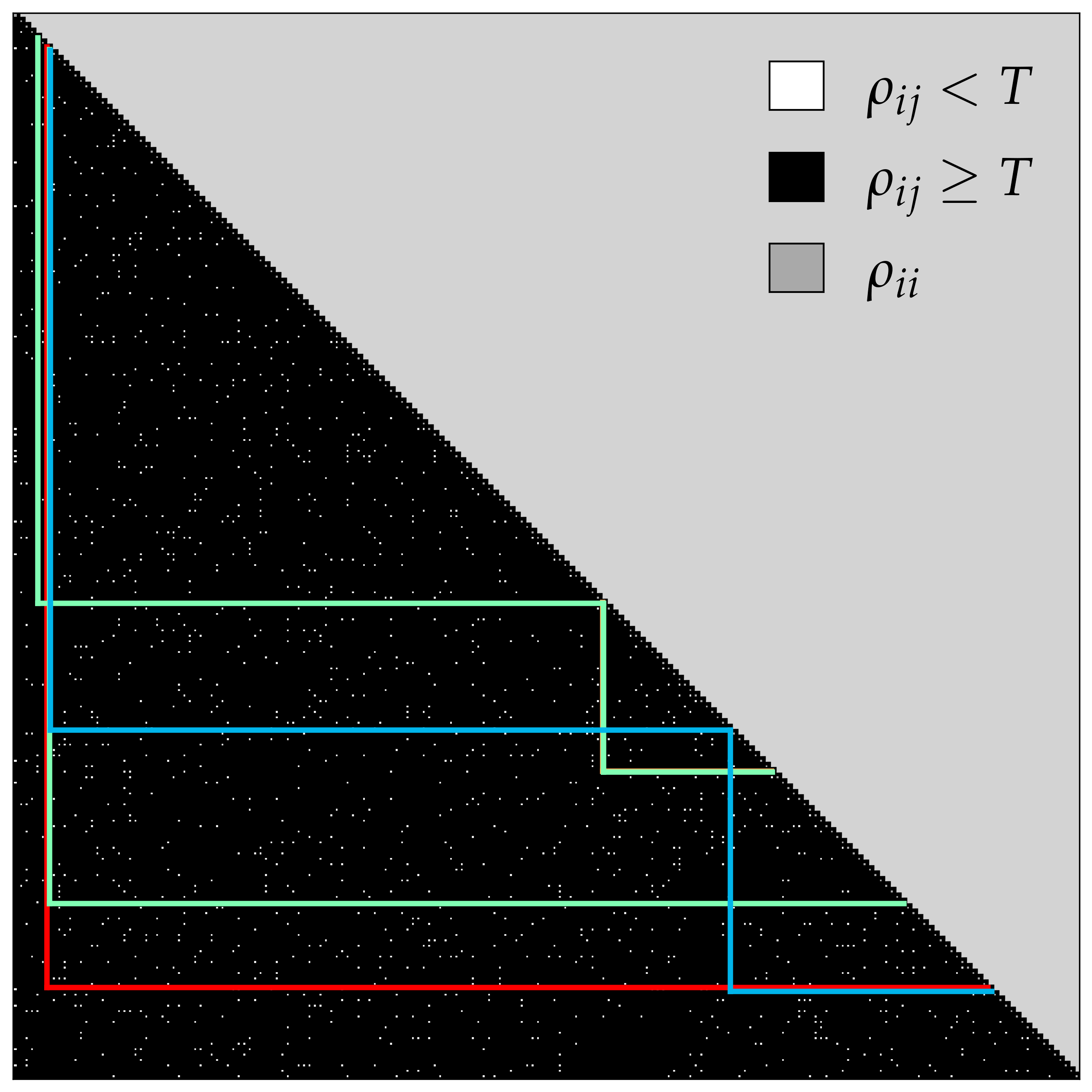
Finally, the dictionary called models is just a container to collect all the models. In the next, let us construct a Binary acceptance matrix and compute the best possible paths

>>> overlap_matrix = pd.read_csv("overlap_matrix.csv", index_col=0)
>>> weights = [models[reg]["llhr"] for reg in list(overlap_matrix.columns)]
>>> bam = pf.BinaryAcceptance(overlap_matrix.to_numpy(), weights=weights, threshold=0.01)

>>> whdfs = pf.WHDFS(bam, top=5)
>>> whdfs.find_paths(runs=len(weights), verbose=False)
>>> plot_results.plot(bam, whdfs)

In the first three lines, we read the overlap matrix, extracted the corresponding weights (llhr), and fed these into the pf.BinaryAcceptance function. We use the WHDFS algorithm to compute the top 5 combinations and plot the resulting binary acceptance matrix with the paths.

Each column and row corresponds to overlap_matrix.columns, and the coloured lines are the chosen paths where the best path can be seen via whdfs.best.path. In this case we find "atlas_susy_2018_31::SRA_H", "cms_sus_19_006::SR25_Njet23_Nb2_HT6001200_MHT350600" and 'cms_sus_19_006::AGGSR7_Njet2_Nb2_HT600_MHT600' regions as best regions to be combined. For the combination, we will use UnCorrStatisticsCombiner and feed the statistical models as input.

>>> regions = [
...      "atlas_susy_2018_31::SRA_H",
...      "cms_sus_19_006::SR25_Njet23_Nb2_HT6001200_MHT350600",
...      "cms_sus_19_006::AGGSR7_Njet2_Nb2_HT600_MHT600"
...  ]
>>> combined = spey.UnCorrStatisticsCombiner(*[models[reg]["stat_model"] for reg in regions])
>>> combined.exclusion_confidence_level(expected=spey.ExpectationType.aposteriori)[2]
>>> # 0.9858284831278277

Note

UnCorrStatisticsCombiner can be used for any backend retrieved via spey.get_backend() function, which wraps the likelihood prescription with StatisticalModel.

UnCorrStatisticsCombiner has exact same structure as StatisticalModel hence one can use the same functionalities. Further mode, we can compare it with the most sensitive signal region within the stack, which can be found via

>>> poiUL = np.array([models[reg]["stat_model"].poi_upper_limit(expected=spey.ExpectationType.aposteriori) for reg in models.keys()])

In our case, the minimum value that we found was from "atlas_susy_2018_31::SRA_H" where the expected exclusion limit can be computed via

>>> models["atlas_susy_2018_31::SRA_H"]["stat_model"].exclusion_confidence_level(expected=spey.ExpectationType.aposteriori)[2]
>>> # 0.9445409288935508

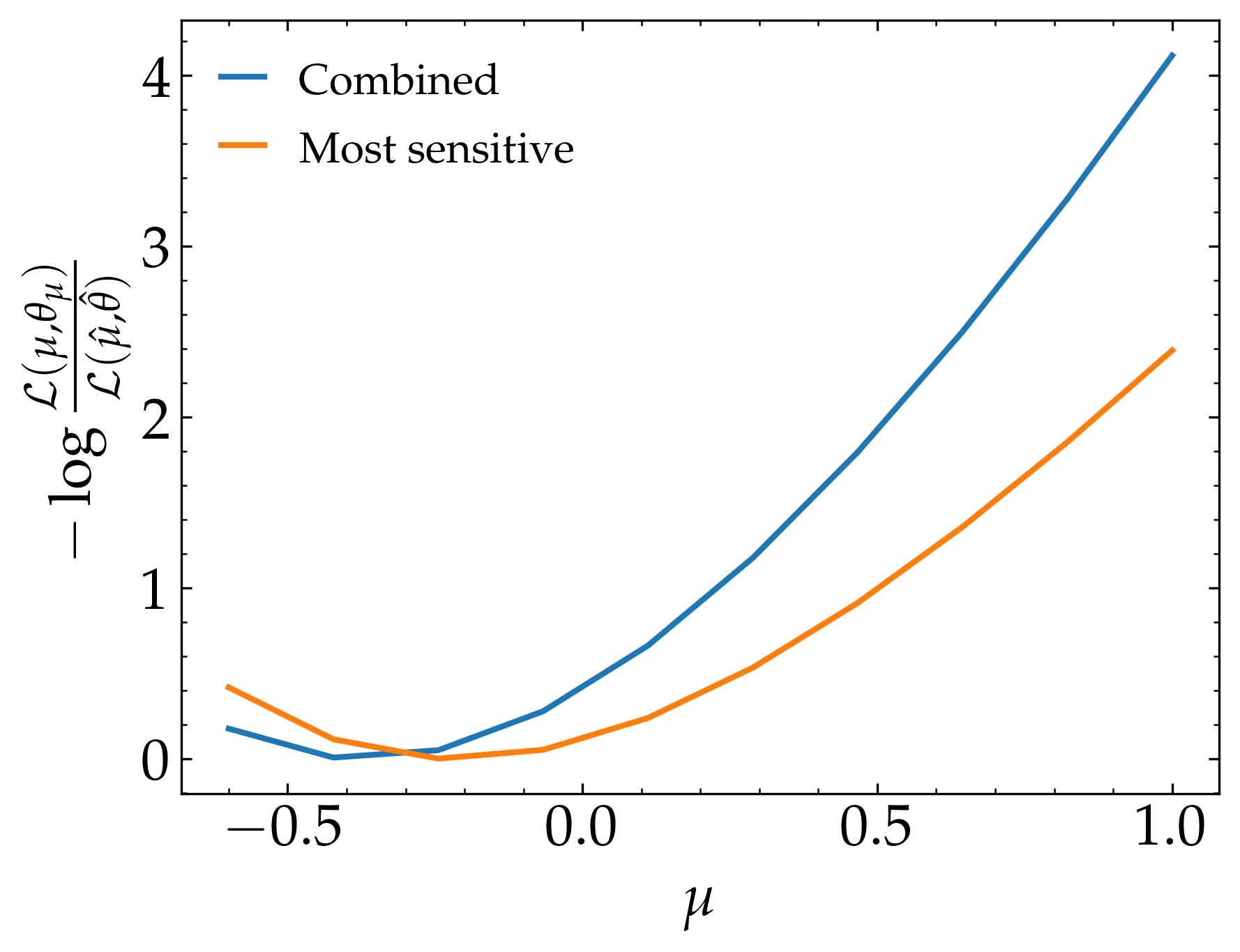
Finally, we can compare the likelihood distribution of the two

>>> muhat_best, maxllhd_best = models["atlas_susy_2018_31::SRA_H"]["stat_model"].maximize_likelihood()
>>> muhat_pf, maxllhd_pf = combined.maximize_likelihood()

>>> poi = np.linspace(-0.6,1,10)

>>> llhd_pf = np.array([combined.likelihood(p) for p in poi])
>>> llhd_best = np.array([models["atlas_susy_2018_31::SRA_H"]["stat_model"].likelihood(p) for p in poi])

>>> plt.plot(poi, llhd_pf-maxllhd_pf, label="Combined" )
>>> plt.plot(poi, llhd_best-maxllhd_best , label="Most sensitive")
>>> plt.xlabel("$\mu$")
>>> plt.ylabel(r"$-\log \frac{ \mathcal{L}(\mu, \theta_\mu) }{ \mathcal{L}(\hat{\mu}, \hat{\theta}) }$")
>>> plt.legend()
>>> plt.show()

which gives us the following result:

Attention

The results can vary between scipy versions and the versions of its compilers due to their effect on optimisation algorithm.