Converting full statistical models to the simplified likelihood framework

Although full statistical models contain all the necessary information to reconstruct the original analysis, it might be computationally costly. Thus, we implement methodologies to convert full likelihoods into simplified likelihood frameworks using "default_pdf.correlated_background" or "default_pdf.third_moment_expansion" models. Details on the simplified models can be found in this link.

This particular example requires the installation of three packages, which can be achieved by using the line below

>>> pip install spey spey-pyhf jax

Methodology

The Simplified likelihood framework contracts all the nuisance parameters into a single bin and represents the background uncertainty as a single source. To capture the correlations between nuisance parameters, one needs to construct a statistical model only from control and validation regions, which is ideally purely dominated by the background, henceforth called the control model \(\mathcal{L}^{c}\). Once nuisance parameters are fitted for the control model without the signal, one can compute the covariance matrix between the nuisance parameters using the Hessian of the negative log probability distribution,

(1)\[\mathbf{V}^{-1}_{ij} = - \frac{\partial^2}{\partial\theta_i\partial\theta_j} \log\mathcal{L}^{\rm c}(0,\theta_0^{\rm c})\]

where \(\theta_0^{\rm c}\) represents the nuisance parameters that maximises \(\mathcal{L}^{\rm c}\) at \(\mu=0\). Covariance matrix \(\mathbf{V}_{ij}\) allows the construction of a multivariate Gaussian distribution \(\mathcal{N}(\theta_0^{\rm c}, \mathbf{V}_{ij})\) where one can sample nuisance parameters, \(\tilde{\theta}\sim\mathcal{N}(\theta_0^{\rm c}, \mathbf{V}_{ij})\), without losing the correlations between them.

Attention

This method is highly dependent on which channels or regions are considered within the control model since this will determine how much of the statistical model is summarised as a multivariate (skewed) Gaussian.

It is essential to note that the nuisance parameters of \(\mathcal{L}^{\rm c}\) does not necessarily need to match the requested statistical model, which might be reduced compared to the entire model. For the sake of simplicity, let us call the requested statistical model \(\mathcal{L}^{\rm SR}\), but bear in mind that this model does not necessarily only contain signal regions. In the case where \(|\theta^{\rm SR}|>|\tilde{\theta}^{\rm c}|\) the remaining nuisance parameters are fitted to maximize \(\mathcal{L}^{\rm SR}\) for a given set of \(\tilde{\theta}^{\rm c}\) and \(\mu=0\). The remaining nuisance parameters that maximise this likelihood are \(\hat\theta^{\rm SR}\).

The simplified likelihood framework requires a covariance matrix, \(\Sigma\), representing the correlations between each bin for the background-only model. To construct the covariance matrix, one can sample from \(\mathcal{L}^{\rm SR}\) using \(\hat\theta^{\rm SR}\) and \(\tilde{\theta}^{\rm c}\);

\[\tilde{n}_b \sim \mathcal{L}^{\rm SR}(\mu=0, \tilde{\theta}^{\rm c}, \hat\theta^{\rm SR})\]

where \(\Sigma = {\rm cov}(\tilde{n}_b)\) and \(n_b=\mathbb{E}[\tilde{n}_b]\). Similarly one can compute third moments of \(\tilde{n}_b\) to extend the model for "default_pdf.third_moment_expansion".

See also

Other techniques have been employed to simplify the full statistical models. One can find such a method in this GitHub repository. Since this approach provides a pyhf compatible dictionary as an output, it can be directly used with the spey-pyhf plug-in without additional modifications. The method presented here is different from their approach.

Usage

A full statistical model can be constructed using a background-only JSON serialised file (usually found in the HEPData entry for a given analysis). Details on constructing a full likelihood through the spey-pyhf interface can be found in this section.

As an example, let us use the JSON files provided for ATLAS-SUSY-2019-08 analysis in HEPData. One can read the file using json package

>>> import json
>>> with open("1Lbb-likelihoods-hepdata/BkgOnly.json", "r") as f:
>>>     background_only = json.load(f)
>>> with open("1Lbb-likelihoods-hepdata/patchset.json", "r") as f:
>>>     signal = json.load(f)["patches"][0]["patch"]

Following the details in previous sections, a statistical model using pyhf interface can be constructed as

>>> pdf_wrapper = spey.get_backend("pyhf")
>>> full_statistical_model = pdf_wrapper(
...     background_only_model=background_only, signal_patch=signal
... )
>>> full_statistical_model.backend.manager.backend = "jax"

where background_only refers to background-only the JSON file retrieved from HEPData and signal refers to a signal patch constructed by the user. Note that the computation of the Hessian in eq. (1) currently requires pyhf’s jax backend, which is ensured by the last line in the snippet above. full_statistical_model can be converted into simplified likelihood by using pyhf.simplify backend.

>>> converter = spey.get_backend("pyhf.simplify")
>>> simplified_model = converter(
...     statistical_model=full_statistical_model,
...     convert_to="default_pdf.correlated_background",
...     control_region_indices=[
...         'WREM_cuts', 'STCREM_cuts', 'TRHMEM_cuts', 'TRMMEM_cuts', 'TRLMEM_cuts'
...     ]
... )

Arguments: (for details see the object reference for Simplify)

• statistical_model: Statistical model constructed using pyhf backend.

• fittype: Flag to choose what type of fit to be performed. Users can choose between "postfit" and "prefit".

• convert_to: Which simplified framework to be used as a baseline for the conversion, default "default_pdf.correlated_background".

• number_of_samples: Sets the number of samples to be generated to construct covariance matrix, \(\Sigma\), for the background bins, default 1000.

• control_region_indices: Usually, the algorithm can pick up the differences between signal, control and validation regions; however, there is no fixed convention in naming, which leads to choosing the wrong channels for the construction of the \(\mathcal{L}^{\rm c}\). One can overwrite the system selection by providing the indices of the control and validation regions within the channel list from the background-only statistical model dictionary. The channel names of the statistical_model can be extracted via list(statistical_model.backend.model.channels) property. For details, see channels.

• include_modifiers_in_control_model: This flag enables the usage of the signal modifiers in the control model. Note that the yield values will still be zero, but the modifiers within the signal model will be copied to the control model. This flag allows the contribution of the signal uncertainties in the nuisance covariance matrix, as shown in eq. (1).

Note

Possible leakage of signal into control or validation regions is disregarded by setting the signal yields to zero while constructing \(\mathcal{L}^{\rm c}\). \(\tilde{n}_b\) does not include the auxiliary data; hence, the final statistical model will only include one uncertainty value per histogram bin.

Validation

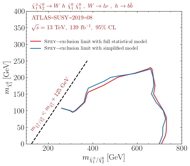
Following the above example, we converted the full likelihood provided for ATLAS-SUSY-2019-08 analysis into the "default_pdf.correlated_background" model (for details see dedicated documentation). The following results use all available channels for the control model while including the modifiers of the signal patchset within the control model. Postfit configuration has been used throughout the simulation. The background yields and covariance matrix of the background-only model have been computed by generating Five hundred samples from the full statistical model. Scan includes 67 randomly choosen points in \((m_{\tilde{\chi}^\pm_1/\tilde{\chi}^0_2},m_{\tilde{\chi}_1^0})\) mass plane.

The following plot shows the observed exclusion limit comparison for the full statistical model and its simplified version, mapped on the "default_pdf.correlated_background" model. Data points only include the ones provided by the ATLAS collaboration within HEPData.

These results can be reproduced by following the prescription described above. Note that the red curve does not correspond to the official results since it is plotted only using 67 points. The official results can be reproduced using the entire patch set provided by the collaboration.

Acknowledgements

This functionality has been discussed and requested during 8th (Re)interpretation Forum. Thanks to Nicholas Wardle, Sabine Kraml and Wolfgang Waltenberger for the lively discussion.